How to Make Swimlanes in Excel: A Step-by-Step Guide

Quick Answer

To make swimlanes in Excel, create one row group for each lane, add task names on the left, put week numbers or dates across the top, shade each lane band, then use conditional formatting or merged cells to create task bars across the timeline.

Use conditional formatting if the file needs to stay editable.
Use merged cells only for a static presentation.
Use horizontal lanes unless you have a specific reason to build vertically.

You can make a swimlane diagram in Excel by turning the worksheet into horizontal lane bands. Each band represents a department, role, vendor, phase, or workstream. Then you add task rows, shade the lane backgrounds, place a timeline across the top, and use either filled cells or conditional formatting to show the task bars.

Excel does not have a dedicated swimlane feature, so this method is best for small, stable workflows. As a rough rule, Excel works well for 10 to 15 tasks across a few lanes. Once the file needs dependencies, frequent schedule changes, or several people editing it at the same time, a dedicated scheduling or diagramming tool will usually be easier to maintain.

Many Excel swimlane tutorials rely on bar charts and reshaped data tables. That can work, but it becomes awkward when dates change. The row-banding method below is more direct and easier to edit.

What You Need Before You Start

Decide two things before building the sheet.

First, define your lanes. These might be departments, roles, vendors, process phases, or teams. Write the lane list before you open Excel. If the lane structure is unclear, the finished diagram will be unclear too.

Second, decide what type of swimlane you need:

Process-flow swimlane: shows which person, team, or department owns each step in a workflow. It usually does not need a timeline.
Gantt-style swimlane: shows tasks across days, weeks, sprints, or milestones. This is the version covered in this guide.

If you need a process-flow diagram, Excel shapes can work for a simple one-time visual, but a diagramming tool such as Lucidchart or Miro will usually be faster. If you need a Gantt-style swimlane, use horizontal lanes with a timeline across the top.

Vertical swimlanes are possible in Excel, but they are harder to maintain. When each lane is a column, long task names quickly force wide columns and make the diagram spread across the page. Use horizontal lanes unless you have a strong reason not to.

Step-by-Step: Building the Layout

This method uses week numbers for the timeline. The same setup also works with real dates, but numbers are easier for a first swimlane.

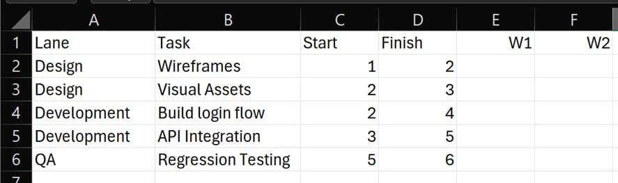
Step 1: Build the header row

Open a blank worksheet.
Click cell A1 and type Lane.
Click cell B1 and type Task.
Click cell C1 and type Start.
Click cell D1 and type Finish.
Click cell E1 and type 1.
Click cell F1 and type 2.
Continue across the row for as many weeks as you need. For a six-week swimlane, enter 1 through 6 in cells E1 through J1.

Do not type W1, W2, or W3 directly into the timeline header cells. Type the numbers only. The conditional formatting rule needs real numbers so it can compare the timeline header against the Start and Finish columns.

To make the numbers display as W1, W2, W3, and so on without turning them into text:

Select the timeline header cells. For a six-week example, select E1:J1.
Right-click the selected cells and choose Format Cells. You can also press Ctrl+1 on Windows or Command+1 on Mac.
In the Format Cells window, choose the Number tab.
Choose Custom from the category list.
In the Type box, enter this format code:

"W"0

Click OK.

The cells will now display as W1, W2, W3, and W4, but Excel still treats them as the numbers 1, 2, 3, and 4. You can confirm this by clicking E1. The cell should show W1 in the worksheet, but the formula bar should still show 1.

If you prefer labels with a space, such as Wk 1 and Wk 2, use this custom format instead:

"Wk "0

This works because Excel custom number formats can display text around a number without changing the underlying numeric value. Microsoft’s guidance is to put added text in quotation marks when creating a custom number format.

Note: if you are using Excel for the web, create the custom number format in the desktop version of Excel. Microsoft’s support page says Excel for the web cannot create custom formats, even though it can open workbooks that already contain them.

Step 2: Enter the task rows

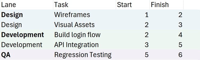
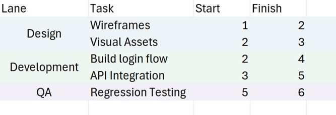
Enter one row per task. For example:

Here’s the example in Text form if you want to quickly copy/paste:

Lane	Task	Start	Finish
Design	Wireframes	1	2
Design	Visual assets	2	3
Development	Build login flow	2	4
Development	API integration	3	5
QA	Regression testing	5	6

In this example, Start and Finish use week numbers. Wireframes starts in week 1 and finishes in week 2, so C2 is 1 and D2 is 2. Build login flow starts in week 2 and finishes in week 4, so C4 is 2 and D4 is 4.

Do not enter W1 or W2 in the Start and Finish columns. Use 1, 2, 3, and so on. The W belongs only in the display formatting for the timeline header.

Step 3: Allocate row bands per lane

Sort or group the task rows by lane so all Design tasks sit together, all Development tasks sit together, and all QA tasks sit together.
Select the full row band for the first lane. In the example above, Design uses rows 2 and 3, so select A2:J3.
Go to Home > Fill Color.
Choose a light, muted background color.
Select the next lane band. In the example, Development uses rows 4 and 5, so select A4:J5.
Apply a different muted fill color.
Select the QA row, A6:J6, and apply another muted fill color.

Keep the lane colors pale. The task bars will sit on top of these lane bands, so the background should not compete with the task-bar color.

Here’s an example of some nice colors to use:

Lane background 1: light blue, #D9E1F2
Lane background 2: light green, #E2EFDA
Lane background 3: light gray, #F2F2F2
Task bars: dark blue, #2F5597
Blocked or urgent tasks: red, #C00000

Step 4: Add the lane labels

There are two ways to handle lane labels. Use one method or the other. Do not mix them in the same file.

Option A: Editable file

For a file that people will sort, filter, copy, or update later, leave the lane name repeated in column A on every task row.

Keep Design in A2 and A3.
Keep Development in A4 and A5.
Keep QA in A6.
Bold the first row of each lane if you want a stronger visual break.

This looks slightly repetitive, but it keeps the sheet much easier to maintain.

Option B: Static presentation file

For a one-time presentation version, you can merge the lane labels.

Select A2:A3 for the Design lane.
Go to Home > Merge & Center.
It should keep the “Design” text from one of the cells (if not, you can add it back in).
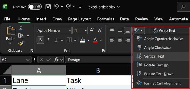
If you want to make the swimlane text vertical in Excel:
- Select the cell, and in the Home tab, click on the text orientation button, and choose either Vertical Text or Rotate Text Up/Down:
- Repeat the same process for A4:A5 for Development.
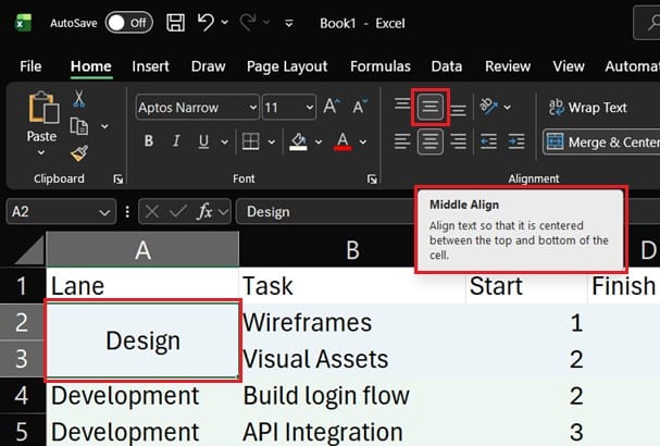
If you want to center your merged horizontal text:
- Select the merged cell
- In the Home Tab, make the vertical alignment of the text centered:
Leave A6 unmerged for QA since it has only one row (in our example).

Use merged lane labels only when the file is mainly for presentation. Merged cells make future sorting and filtering harder.

Step 5: Place the task bars

There are two practical ways to place task bars. The conditional formatting method is better for an editable file. The merged-cell method is better for a static visual.

Option A: Conditional formatting method

Use this method when Start and Finish values may change later.

Select the timeline grid, not the whole table. In this example, select E2:J6.
Go to Home > Conditional Formatting > New Rule.
Choose Use a formula to determine which cells to format.
In the formula box, enter:

=AND(E$1>=$C2,E$1<=$D2)

Click Format.
Go to the Fill tab.
Choose a task-bar color that is darker than the lane background.
Click OK.
Click OK again to apply the rule.

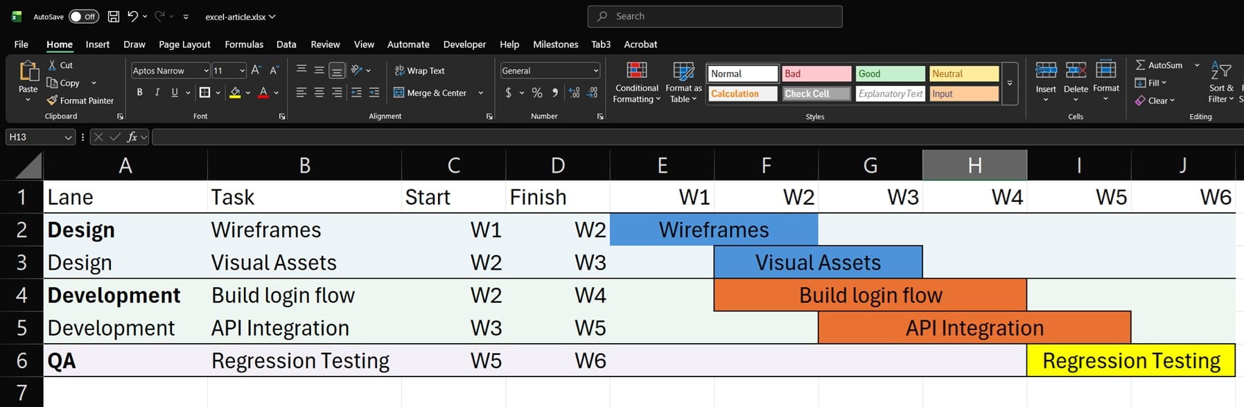
Excel will now shade each task’s active weeks automatically. For example, Build login flow has Start = 2 and Finish = 4. Because the week headers are 1, 2, 3, 4, 5, and 6, Excel shades the cells for weeks 2, 3, and 4.

Here’s an example of what that formula outputs for the example that I’ve built:

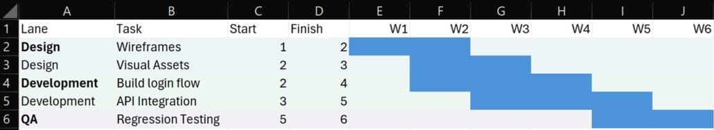
The formula works like this:

E$1 checks the week number at the top of the current timeline column.
$C2 checks the Start value for the current task row.
$D2 checks the Finish value for the current task row.
AND(...) applies the fill only when the timeline week is greater than or equal to Start and less than or equal to Finish.

The dollar signs matter. In E$1, the row number stays locked to row 1 while the column moves across the timeline. In $C2 and $D2, the columns stay locked to Start and Finish while the row changes for each task.

If your timeline starts somewhere other than column E, adjust the formula. For example, if the first timeline column is G, the formula should start with G$1. If your first task row is row 3, use $C3 and $D3.

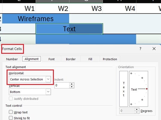
Note: If you use this method, and you want to add labels to the bars, you will need to “Center Across Selection” by selecting all the cells of a bar, Right Click > Format Cells (or pressing CTRL+1), and choose Horizontal:

Option B: Merged-cell method

Use this method only for a static presentation file. This is more manual but also less reliant on a formula.

Look at the task’s Start and Finish values.
Find the matching week columns in the timeline.
Select the cells across that task’s time span.
Go to Home > Merge & Center. Use Merge Cells if you do not want Excel to center the text automatically.
Apply a task-bar fill color through Home > Fill Color.
Type the task name inside the merged bar if you want the label to appear directly on the bar.
Turn on Wrap Text if the label is long.

For example, Build login flow is in row 4 and runs from week 2 through week 4. Since week 1 is in column E, week 2 is in column F, week 3 is in column G, and week 4 is in column H. Select F4:H4, merge those cells, apply a fill color, and type Build login flow.

Step 6: Separate the lanes with borders

Select the last row of the first lane. In the example, Design ends on row 3, so select A3:J3.
Go to Home > Borders.
Choose Thick Bottom Border.
Repeat this for the last row of each lane. Development ends on row 5, so select A5:J5. QA ends on row 6, so select A6:J6.

Use borders instead of extra blank rows if the file needs to stay sortable or filterable. Blank spacer rows are fine for a presentation file, but they can get in the way when the worksheet is edited later.

Step 7: Freeze the header and labels

Click cell E2.
Go to View > Freeze Panes > Freeze Panes.

This freezes row 1 and columns A through D. That means the Lane, Task, Start, Finish, and timeline header stay visible while you scroll across the schedule. Microsoft explains Freeze Panes this way: Excel freezes the rows above and the columns to the left of the selected cell. That is why E2 is the correct cell here.

Formatting Tips That Make It Readable

Limit the lane colors. Four or five muted background colors are usually enough. If every lane uses a saturated color, the task bars become harder to read.

Use consistent type sizes. A 10 or 11 pt font works well for task labels. Lane names can be slightly larger and bold. Turn on Wrap Text for long task names so they do not spill into neighboring cells.

Add a small legend in an unused corner of the sheet. If color represents status, priority, owner, or lane type, say so clearly. Anyone opening the file later should not have to guess what a color means.

Before sharing the swimlane, check the print layout. Go to Page Layout > Print Area > Set Print Area, then use Page Setup to fit the diagram to one page wide. Excel swimlanes often become unreadable when lane bands split across printed pages.

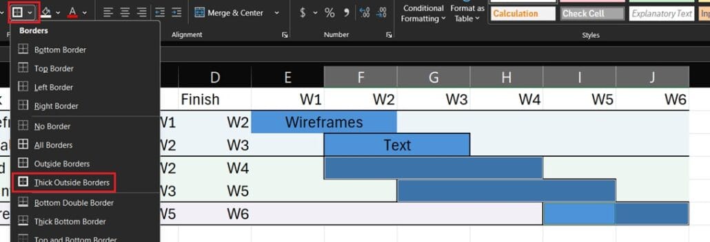
You can add borders to the actual gantt bars as well. The easiest way is probably to hold CTRL + click/drag to select all of your gantt bars, and then in the Home Tab go to Border -> Thick Outside Borders. This should place borders around all of the bars:

Where Excel Swimlanes Break Down

Excel swimlanes are useful as lightweight planning views and presentation visuals. They are not full scheduling systems.

The limits show up quickly when the swimlane needs dependencies, resource loading, recurring status updates, or frequent date changes. With merged cells, every schedule change requires manual cleanup. With conditional formatting, date changes are easier, but Excel still will not manage dependencies or resource conflicts for you.

Modern Excel co-authoring helps with collaboration, but it does not solve the maintenance problem created by merged cells, manual colors, and shape-heavy layouts. The more people editing the file, the more important it is to keep the structure simple.

For schedule-driven work, consider a dedicated planning tool. Smartsheet is better suited to team-managed project plans with row hierarchies, Gantt views, and dependencies. TeamGantt is built around Gantt planning, with task groups, subgroups, milestones, and dependency tracking. Microsoft Project is better for complex schedules. Milestones Professional is useful when the main deliverable is a polished timeline report.

For process-flow swimlanes, consider Miro, FigJam, Lucidchart, or Visio. These tools handle boxes, connectors, and lane structures more naturally than Excel.

For a free or lightweight option, Google Sheets can reproduce the same row-banding and conditional-formatting approach. It still has the same basic limitation: it can show a schedule, but it does not manage the schedule logic for you.

Common Mistakes Worth Avoiding

Using merged cells in a file that needs editing. Merged cells are fine for a static visual, but they make sorting, filtering, copying, and updating harder. If the file needs to stay usable, repeat the lane name in each row and use conditional formatting for task bars.

Typing week labels as text. Labels like “Wk 1” look clean, but they behave like text. Use real numbers or real dates, then format the cells to display the label you want.

Freezing the wrong cell. If your timeline starts in column E, select E2 before using Freeze Panes. Selecting B2 freezes only row 1 and column A.

Building a bar chart when a grid will do. Excel bar charts can be adapted into Gantt-style visuals, but they require extra data setup and become harder to maintain when schedules change. For a simple swimlane, the grid method is usually easier.

Skipping the legend. If color means anything, document it. A small legend prevents confusion and makes the file easier to hand off.

Summary

Use Excel for a small, stable swimlane that needs to show tasks across lanes and time. Use merged cells when you need a one-time presentation. Use conditional formatting when the file needs to be edited after the first meeting.

If the swimlane starts acting like a real schedule, move it out of Excel. Dependencies, resource planning, weekly updates, and multi-person editing are signs that a dedicated tool will save time.